Interdependence of returns across multiple strategies

When constructing a portfolio, it's common to see low pairwise correlations among strategies - say, around 0.2. However, this number may not fully capture the underlying dependency between strategies, especially when they're built to exploit similar market tendencies, such as intraday trends. In this article, I explore how strategies can be interdependent, and why relying solely on correlation can be misleading when assessing risk.

Shared Underlying Market Factor

Even if day-to-day return correlations appear modest, strategies might still be exposed to the same market regime. When the regime shifts, strategies may suffer simultaneously, even if their daily movements do not appear to be in lockstep. In essence, they are interdependent in terms of their underlying risk factors.

Limitations of Correlation as a Measure

Correlation primarily measures linear relationships and can miss nuances such as tail dependencies (simultaneous large losses) or regime-specific behaviors. In markets characterized by heavy whipsaws and reversals, the distribution of returns can be non-Gaussian, which means that a simple Pearson correlation might understate the true risk of simultaneous losses.

Regime Sensitivity

Strategies with low average correlation might become correlated when the underlying market regime changes. In other words, they become correlated at the worst possible time (during adverse market conditions). This phenomenon underscores the importance of looking beyond correlations to understand the true interdependence among strategies.

Alternative Measures

To capture these dependencies more accurately, consider the following alternative measures:

Co-Movement Measures: Dynamic correlations, rolling correlations, and cointegration provide insight into how relationships change over time and under different market conditions.

In the code snippets, returns_df is a pandas DataFrame where each column represents a different strategy and each row corresponds to the return over a given time period—such as daily or weekly. This format allows us to easily compute various correlation metrics between strategies.

overall_corr = returns_df.corr().loc["StrategyA", "StrategyB"]
rolling_corr = returns_df["StrategyA"].rolling(window=10).corr(returns_df["StrategyB"]

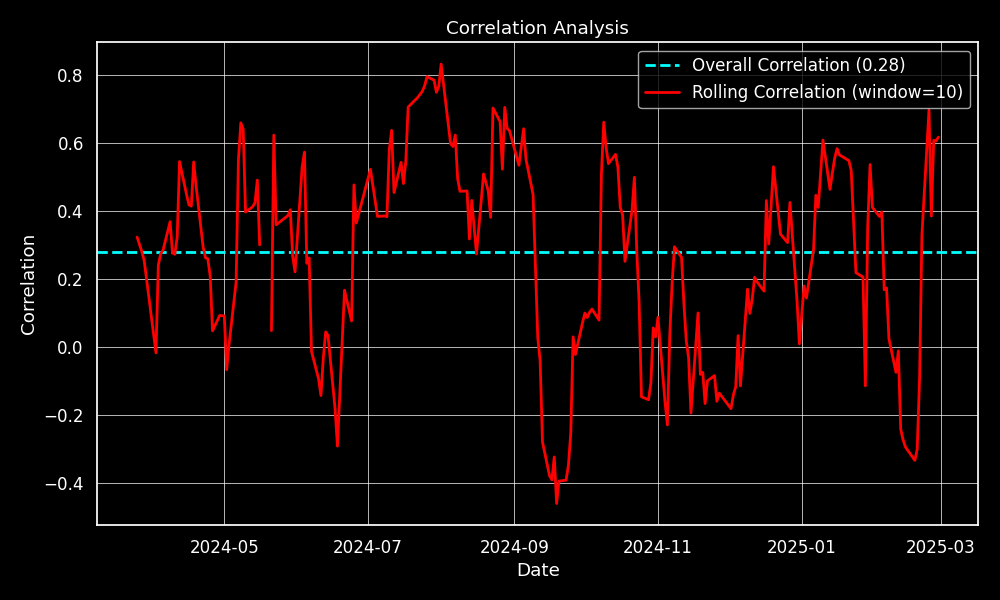
The overall correlation between StrategyA and StrategyB is 0.28. However, when we look at the 10-day rolling correlation, we see that their relationship can be considerably stronger or weaker in the short term.

Tail Dependence: Focuses on the joint behavior in the extremes, which is critical for understanding the risk of simultaneous large losses.

def tail_dependency(returns_df, quantile=0.1):
    """
    Compute the tail dependency between pairs of strategies.
    """

    thresholds = returns_df.quantile(quantile)

    # Find tail events (big losses)
    tail_events = returns_df.lt(thresholds, axis=1).astype(float)
    tail_counts = tail_events.sum(axis=0)

    # Compute pairwise simultaneous tail events
    both = tail_events.T.dot(tail_events)

    # P(strategy1 in tail | strategy1 or strategy2 in tail)
    row_counts = tail_counts.values.reshape(-1, 1)
    col_counts = tail_counts.values.reshape(1, -1)
    tail_dep_matrix = 0.5 * (both.values / row_counts + both.values / col_counts)

    # Set the diagonal values to 1.0
    np.fill_diagonal(tail_dep_matrix, 1.0)

    return pd.DataFrame(tail_dep_matrix, index=returns_df.columns, columns=returns_df.columns)

Factor Analysis: Decomposes strategy returns into common underlying factors, helping to identify whether strategies are truly diversified or merely different manifestations of the same risk exposure.

Conditional Loss Probability: This metric measures the likelihood that strategy A loses money on a given day, given that strategy B loses money on that same day. By focusing on downside risk, it provides a clearer picture of how often two strategies experience losses simultaneously.

Below is an example of how to calculate conditional loss probability:

def conditional_loss_probability(returns_df):
    """
    Compute the conditional loss probability between pairs of strategies.
    """

    loss = (returns_df < 0).astype(float)

    # Number of loss days for each strategy
    total_losses = loss.sum(axis=0)
    total_losses = total_losses.replace(0, np.nan)

    # Pairwise simultaneous losses
    both_losses = loss.T.dot(loss)

    # Convert total_losses to numpy arrays
    row_losses = total_losses.values.reshape(-1, 1)
    col_losses = total_losses.values.reshape(1, -1)

    cond_matrix = 0.5 * (both_losses.values / row_losses + both_losses.values / col_losses)

    # Set the diagonal values to 1.0
    np.fill_diagonal(cond_matrix, 1.0)

    return pd.DataFrame(cond_matrix, index=returns_df.columns, columns=returns_df.columns)

Conclusion

While low return correlations might initially suggest that strategies are diversified, the interdependence of returns can be hidden behind these numbers. By considering alternative metrics such as tail dependence, co-movement measures, factor analysis, and conditional loss probability, we gain a more complete picture of the true risks in a portfolio.